[ Operation Guide ]
■ Numerical Integration
In this application, numerical integration using the trapezoidal rule is used to calculate velocity data from acceleration data and position data from velocity data.
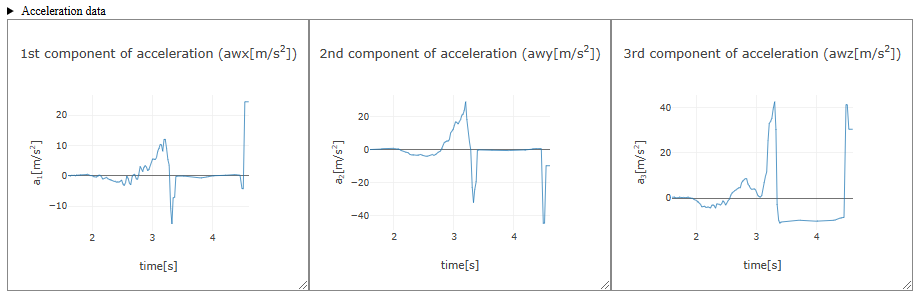
As an example, after loading acceleration data and setting the time domain for analysis, an acceleration graph for each component, as shown below, is obtained (x, y, and z components of the acceleration of projectile motion). Clicking "▶ Acceleration data" just above the graph displays a table of acceleration data for the specified time domain (clicking again closes the table).
The equation to calculate velocity $\vec{\bm{v}}$ from acceleration $\vec{\bm{a}}$ is $$\vec{\bm{v}}(t)=\int_{t_0}^{t}\!\vec{\bm{a}}\,dt+\vec{\bm{v}}_0,$$ so the initial velocity $\vec{\bm{v}}_0$ (velocity $\vec{\bm{v}}(t_0)$ at time $t=t_0$) must be set before performing numerical integration.
When smoothing acceleration data (e.g., Smoothing by Fourier transform, Smoothing by least-squares approximation), you can choose from "Original data," "Smoothed data," or "Difference data" as the acceleration data for numerical integration.
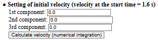
In the initial velocity setting field, input the initial velocity $\vec{\bm{v}}(t_0)$ for each component at the starting time set in the time domain for analysis. Generally, initial velocity values are rarely known beforehand, so measurements can start from rest, and the initial velocity can be set to zero (default is 0.0).
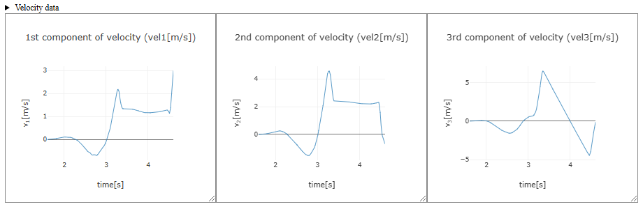
After setting the initial velocity, clicking the "Calculate velocity (numerical integration)" button performs numerical integration of the acceleration data over the specified time domain to calculate velocity data. The velocity graph for each component is displayed as shown below. Clicking "▶ Velocity data" just above the graph displays a table of velocity data obtained through numerical integration (clicking again closes the table).
Similarly, the equation to calculate position $\vec{\bm{r}}$ from velocity $\vec{\bm{v}}$ is $$\vec{\bm{r}}(t)=\int_{t_0}^{t}\!\vec{\bm{v}}\,dt+\vec{\bm{r}}_0,$$ so the initial position $\vec{\bm{r}}_0$ (position $\vec{\bm{r}}(t_0)$ at time $t=t_0$) must be set before performing numerical integration.
When smoothing velocity data (e.g., Smoothing by Fourier transform, Smoothing by least-squares approximation), you can choose from "Original data," "Smoothed data," or "Difference data" as the velocity data for numerical integration.
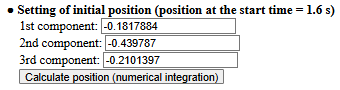
In the initial position setting field, input the initial position $\vec{\bm{r}}(t_0)$ for each component at the starting time set in the time domain for analysis (default is 0.0, setting the initial position at the origin at the starting time). In the example, the initial position is set such that the moment of throwing a smartphone in projectile motion (time = 3.37 seconds) corresponds to the origin.
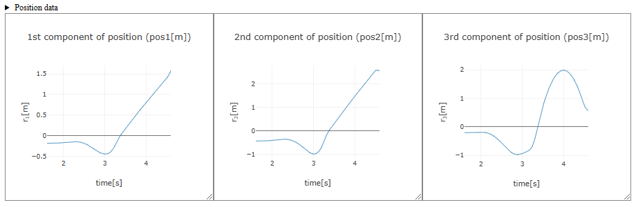
After setting the initial position, clicking the "Calculate position (numerical integration)" button performs numerical integration of the velocity data over the specified time domain to calculate position data. The position graph for each component is displayed as shown below. Clicking "▶ Position data" just above the graph displays a table of position data obtained through numerical integration (clicking again closes the table).
Once position data is obtained through numerical integration, proceed to outputting acceleration, velocity, and position data. If multiple components are analyzed (by selecting multiple columns in acceleration selection), proceeding to data output generates graphs of acceleration, velocity, and position with overlaid plots of multiple components.