Trapezoidal rule for numerical integration

Trapezoidal rule

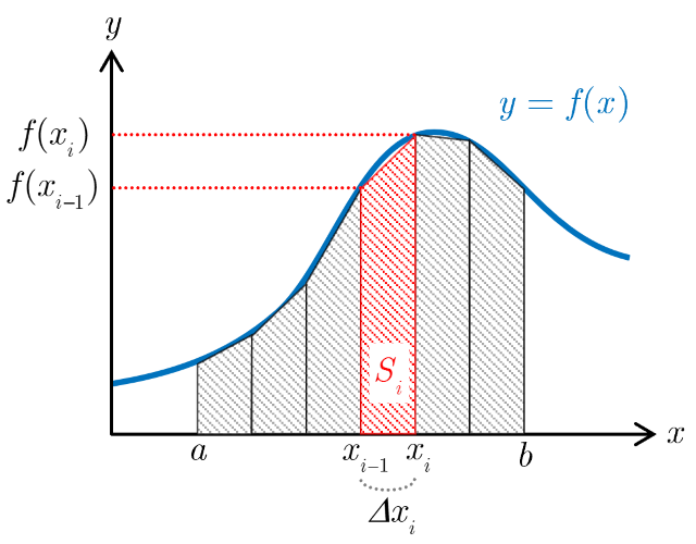
If the acceleration of an object is obtained as numerical data, its velocity is computed approximately by numerical integration. This analysis application employs the trapezoidal rule for numerical integration. For a function $y=f(x)$, given $n+1$ points $(x_i,\,f(x_i))$ in the interval $[a,b]$ ($i=0$ to $n$, $x_0=a$, $x_n=b$), numerical integration using the trapezoidal rule gives the following. The area of the $i$-th subinterval $[x_{i-1},\,x_i]$, where the interval $[a,b]$ is divided into $n$ parts, is obtained from the trapezoidal area formula as, $$S_i=\frac{1}{2}\left\lbrace f(x_{i-1})+f(x_i)\right\rbrace\Delta x_i\ \ \ \ \ \ (i=1\sim n),$$ where $\Delta x_i=x_i-x_{i-1}$ indicates the width of the subinterval $[x_{i-1},\,x_i]$. Thus, if the subinterval width $\Delta x_i$ is sufficiently small, the integral over the interval $[a,b]$ can be approximated as $$\int_{a}^{b}f(x)dx\approx S_1+S_2+\cdots+S_n=\sum_{i=1}^{n}S_i.$$